> OctoPerf's load testing - Report items legends and metrics documentation page. How to add, remove, edit metrics of report items using their legend.
Source: https://api.octoperf.com/doc/analysis/edit-bench-report/metrics-selection/
# Metrics selection
The metrics selection page allows you to change the report items configuration. It can be accessed from any report item through a click on its name/header or on each one of the metrics in its legend:
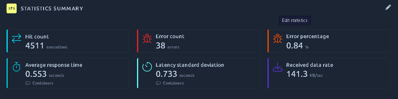
Upon editing any report item, you will be redirected to the metrics selection page in a new tab:
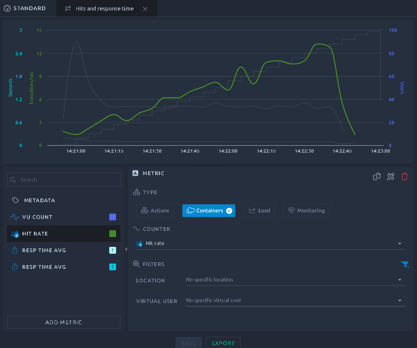
## Add/remove a metric
The bottom left section offers a list of all the metrics configured on this report item, you can click one to select it. You can then use a handful of contextual actions available on the currently selected metric:
| Icon | Name | Description |
|-------------------------------------------------------|---------------|----------------------------------------------------------------------------------------------------------------------------------------------------------------------------------------------------|
| { .off-glb } | Add Metric | Adds a new metric to the report item. |
| { .off-glb } | Color Picker | Opens a color picker to override the default metric color. |
| { .off-glb } | Move Up | Moves the metric up in the report item. |
| { .off-glb } | Move Down | Moves the metric down in the report item. |
| { .off-glb } | Duplicate | Add a duplicate of this metric to the graph. Use it if you want to add a similar metric but with a different filter. |
| { .off-glb } | Apply filters | Applies the filters of the currently selected metric to every other metric that supports them, the *Hit* / *Container* selection included. A metric a filter does not apply to is left untouched, so monitoring metrics keep the counter they measure. The button is disabled when the selected metric has nothing to propagate. |
| { .off-glb } | Delete | Removes this metric from the report item. |
| { .off-glb } | Export Item | Export this report item. Refer to the [dedicated page](https://api.octoperf.com/doc/analysis/export-bench-report/export-report-items/) for more info. |
| { .off-glb } | Save | Save the current configuration and update the report. |
!!! note
**Metadata** allows you to update the report item metadata and as such cannot be removed or duplicated.
## Curve header
In the list of curves, the header of each curve shows at a glance what is customized on it:
| Indicator | Meaning |
|-------------------|----------------------------------------------------------------------------------------------------------------------------------------------------------------------------------------------|
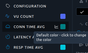
| **Color swatch** | Click it to open the color picker. Its tooltip tells whether the curve uses its default color or a custom one, and how many filter tags apply to the curve. |
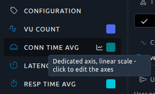
| **Axis icon** | Shown when the axis of the curve is customized: dedicated axis, logarithmic scale, or both. Click it to open the **Configuration** panel directly on the [Y axes](#axes) box. |
| **Gauge** | Shown when the [APDEX](#apdex) thresholds of the curve are customized. Its tooltip gives the _Satisfying_ and _Tolerating_ delays. |
Tooltips of the axis icon (left) and of the color swatch (right) on a detached curve:
## Curve highlighting
The chart at the top of the page helps you see which curve you are working on.
The curve being edited is drawn thicker. The other curves fade but keep their colors, so every curve stays readable:
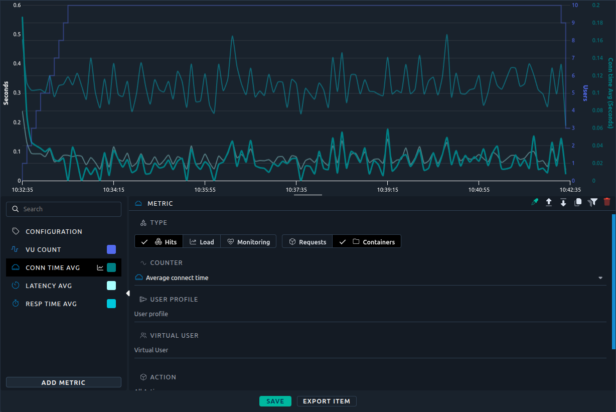
Hovering a curve in the list highlights it and greys out the others. When you move the mouse away, the chart highlights the edited curve again:
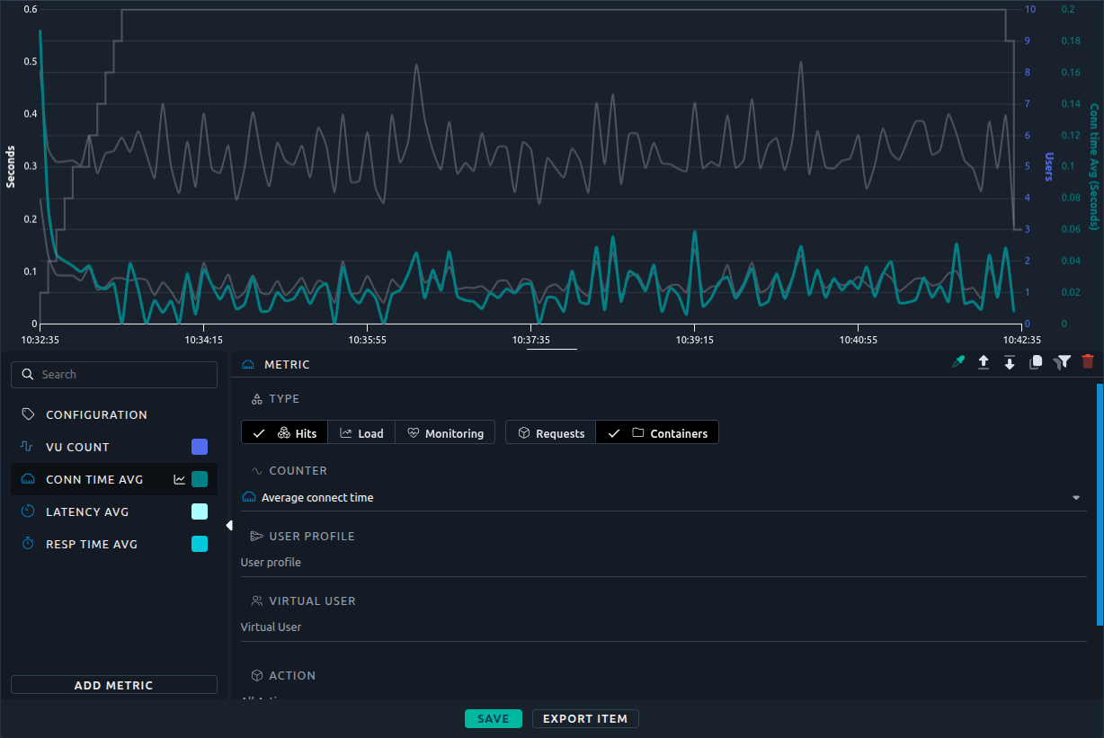
When the **Configuration** panel is open, all curves are drawn normally.
## Multi term filter
Filters on location or virtual user contents are multi term filter, meaning you can select multiple elements from the list:
!!! warning
In order for the filter to work as expected, make sure to filter elements of similar nature.
In other words, do not mix :
- Regions with Injectors,
- Containers with requests.
## Metric type
### Load
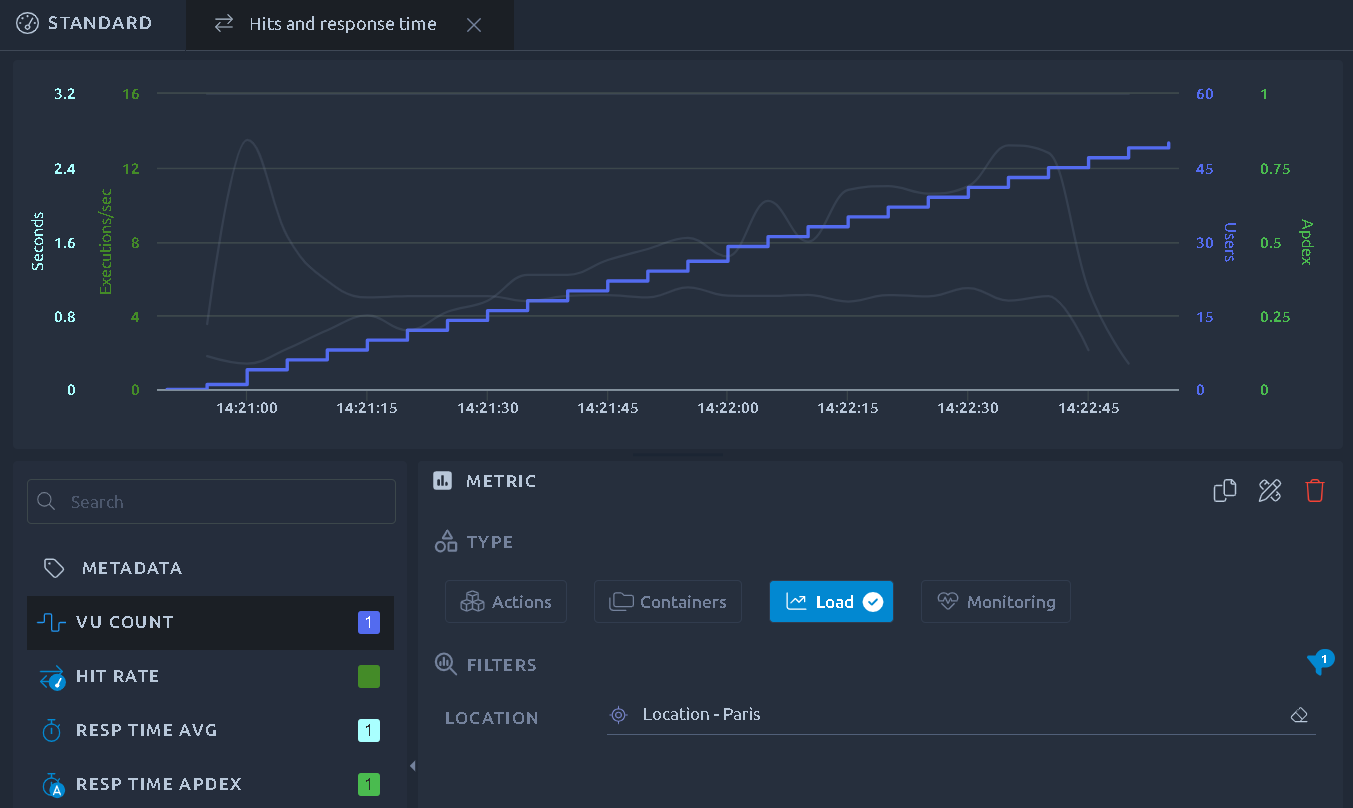
This option allows you to display values related to the number of users running during your test:
!!! note
The load is a real metric reported by the load generators and not a reconstruction based on your test profile. If a virtual user stops during your test you will be able to see it through this metric.
### Actions/containers
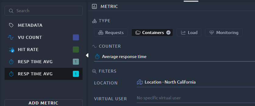
This is what we call hit metrics:
- Requests refers to HTTP requests metrics,
- Containers to everything else, including plugins and other custom elements.
The [complete list of hit metrics is described here](https://api.octoperf.com/doc/analysis/edit-bench-report/performance-metrics/#hit-metrics).
Depending on the report item, you can select various filters:
* Location: The geographical region or the load generator,
* Virtual user: The virtual user used,
* User profile: Which user profile of the scenario the measurements come from. The same virtual user can be played by several user profiles, and the *Set Up* and *Tear Down* phases of a profile appear as their own entries,
* Action: Once you've selected a virtual user you can also filter on a single action/container.
!!! note
Since OctoPerf `17.0.0`, a measurement is attached to your actions and virtual users by their **name and their position**, not by an internal identifier.
!!! note
Some metrics (like Received Bytes) are not available for containers. Selecting those will switch you to **Requests** instead.
### K6 virtual users
The hit metrics of a [K6 Virtual User](https://api.octoperf.com/doc/design/create-virtual-user/import-k6-scripts/) come in three kinds, which the **K6** filter picks once a virtual user is selected:
- `SCRIPT`: the entrypoint of the Virtual User. Its **Containers** are the iterations of the script, its **Requests** the checks and the errors of the script,
- `GROUP`: a `group` block of the script, a container of the requests it runs,
- `REQUEST`: a request of the script, whatever its [protocol](https://api.octoperf.com/doc/design/edit-virtual-user/action-types/k6-actions/k6-protocols/): HTTP, gRPC, WebSocket, SQL, Redis or Kafka.
Combine the **K6** filter with **Requests** or **Containers**: the requests of a `SCRIPT` are its checks, not its HTTP requests. The **Engine** filter keeps the measurements of one engine, JMeter, Playwright or K6, in a scenario that mixes them.
### Custom metrics
The **Custom** type shows the metrics that the scripts record themselves, the `Trend`, `Counter`, `Gauge` and `Rate` of a K6 script, the verdicts of the K6 thresholds, and the [Core Web Vitals](https://api.octoperf.com/doc/design/edit-virtual-user/action-types/playwright-actions/playwright-spec-action/#core-web-vitals) of Playwright scripts. Pick one metric by its name in the **Metric** filter, then the statistic to show:
| Metric | Value |
|--------|-------|
| Average, Minimum, Maximum custom metric value | the average, lowest and highest value recorded |
| Custom metric total | the sum of the values |
| Custom metric value count | the number of values recorded |
| Custom metric rate | the sum of the values per second |
When the scripts of a test declare custom metrics or thresholds, its default report gets a **Custom Metrics** section, right after the **Errors** one: a statistic table with one row per metric name, and each of the statistics above as a column. **Create Line Chart** on a row charts its metric over time.
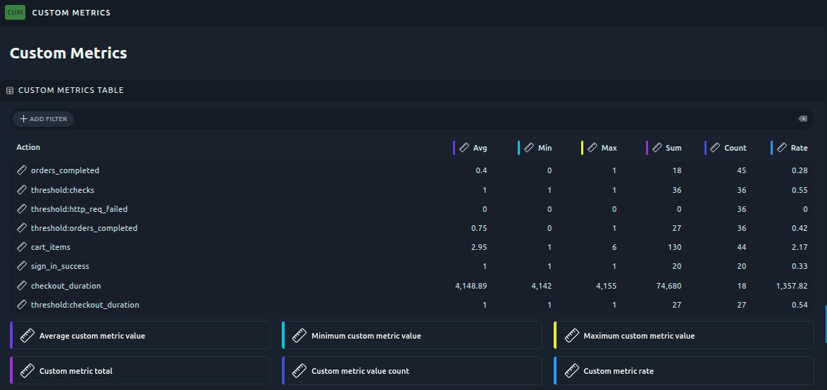
A threshold of the script shows as the metric `threshold:`, `threshold:http_req_duration` for instance: a rate, at 1 while every threshold of that metric holds and at 0 once one fails, per load generator and since the start of the test.
The Web Vitals of a Playwright script are recorded per action: the **Action** filter keeps the Web Vitals of one page load. K6 metrics carry no action, so a custom metric filtered by action leaves them out. When you copy the filters of a performance metric to a custom metric, its action filter is copied too.
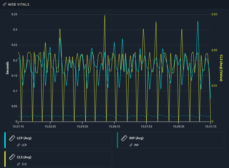
When a test runs a Playwright Virtual User, its default report gets a **Web Vitals** line chart after the **Custom Metrics Table**, with `LCP` and `INP` on the time axis and `CLS` on an axis of its own. The **Web Vitals** button of the [Results Table](https://api.octoperf.com/doc/analysis/edit-bench-report/report-items/results-table/#web-vitals) creates the same chart for a single action.
**Unit of a custom metric**
A custom metric measured in time, such as `LCP` or a K6 `Trend` of durations, or in data, such as the bytes sent, is shown in its unit: milliseconds or bytes, with the axis formatted accordingly. Curves of the same unit share an axis. The editor takes the unit from the metric itself when you pick it. A metric with no unit, such as `CLS` or a counter, is shown as a plain number on an axis of its own.
!!! info
Custom metrics are only shown in line charts and statistic tables, and the editor warns when the metrics picked mix kinds or units. Each load generator reports at most 100 metric names: see [K6 limits](https://api.octoperf.com/doc/design/edit-virtual-user/action-types/k6-actions/k6-limits/#test).
### Monitoring metrics
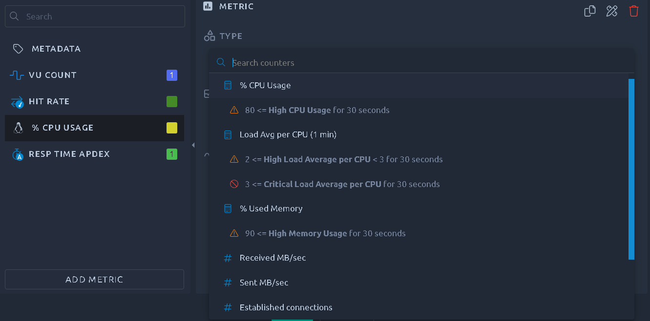
By default [monitoring metrics are available for each load generator](https://api.octoperf.com/doc/analysis/edit-bench-report/performance-metrics/#monitoring-metrics-list) machine used during the load test. You may have many other monitors available if you configured monitoring connections for the server infrastructure under test.
Filters do not apply to Monitoring metrics.
!!! info
More information about the monitoring usage are available in the [Threshold Usage page](https://api.octoperf.com/doc/monitoring/threshold-usage/).
## Y axes { #axes }
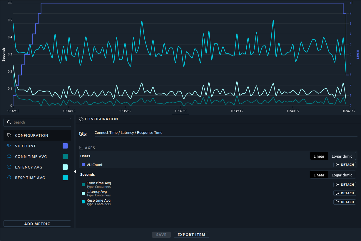
By default, all the curves that share a unit also share a Y axis. When their values have very different magnitudes, the smallest curves are crushed at the bottom of the chart. A typical case is the minimum, average and maximum response times shown together, or a small monitoring counter next to a large one.
The **Y axes** box of the **Configuration** panel lets you fix this. It lists the Y axes of the chart, one block per axis, with the curves each axis carries. Shared axes come first, dedicated axes after them.
In the example below, the average connect time shares the _Seconds_ axis with the latency and the response time. Its values are so small that the curve is hard to read:
!!! note
The **Y axes** box is available for [line charts](https://api.octoperf.com/doc/analysis/edit-bench-report/report-items/line-chart/) (including the ones created from monitoring), [percentiles charts](https://api.octoperf.com/doc/analysis/edit-bench-report/report-items/percentiles-chart/) and [bar charts](https://api.octoperf.com/doc/analysis/edit-bench-report/report-items/bar-chart/). Bar charts only support the scale setting.
### Linear or logarithmic scale
Each axis can be **Linear** (the default) or **Logarithmic**. The scale applies to all the curves carried by the axis.
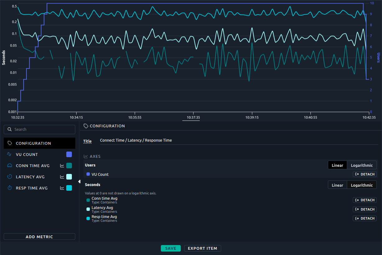
A logarithmic scale gives the same room to each order of magnitude (1, 10, 100, 1000...). Curves of 50 ms and 5 s become readable on the same axis. Here the _Seconds_ axis is logarithmic, and the three curves are readable:
!!! warning
On a logarithmic axis, values at 0 cannot be drawn and are left out of the curve. The **Y axes** box reminds you of it under the axis. This is why the logarithmic scale is never applied automatically.
### Dedicated axis
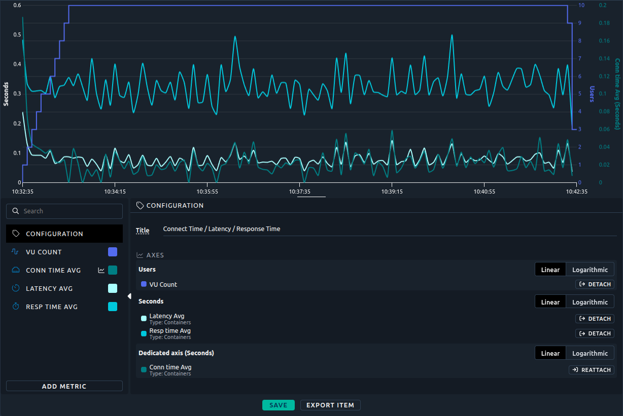
Click **Detach** next to a curve to move it to an axis of its own. The curve is no longer constrained by the scale of the other curves of its unit. It then appears in a **Dedicated axis** block, which has its own scale setting.
Here the average connect time is detached. Its axis, titled **Conn time Avg (Seconds)**, goes from 0 to 1.4 seconds, while the _Seconds_ axis goes up to 6, and the curve uses the full height of the chart:
Click **Reattach** to put the curve back on the shared axis of its unit. The curve then uses the scale of the shared axis again.
For example, to show the minimum, average and maximum response times together, detach the minimum response time: it gets its own axis, and every curve uses the full height of the chart.
### On the chart
- A dedicated axis is titled after its curve, followed by the unit, for example **Conn time Avg (Seconds)**.
- Dedicated axes alternate between the left and right sides of the chart.
- A dedicated axis fits its curve: a percentage that never goes above 80 gets an axis from 0 to 80, not from 0 to 100. The thresholds of that curve follow its axis.
- An axis that carries a single curve takes the color of that curve, custom color included. An axis shared by several curves is drawn in the text color.
The axis settings are saved with the report item, kept in [report templates](https://api.octoperf.com/doc/analysis/edit-bench-report/templates/), and apply to the [PDF export](https://api.octoperf.com/doc/analysis/export-bench-report/).
## APDEX
A particular hit metric, the APDEX, requires additional configuration: the _Satisfying_ and _Tolerating_ delays.
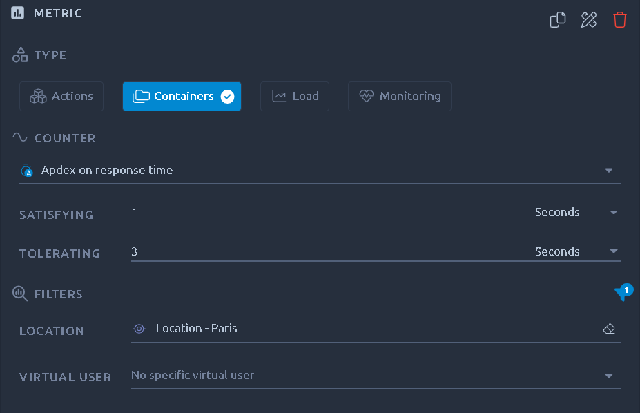
The default values are based upon the ones in the [configuration panel](https://api.octoperf.com/doc/analysis/edit-bench-report/configuration/#apdex).